Physics Sample Paper Review Your roadmap to a perfect 70 in Physics.

Question Distribution & Your Strength

Chapter	Paper Marks	Your Accuracy	Strength
Electrostatics	8	90%	Strong
Current Electricity	7	60%	Moderate
Magnetism & Matter	5	70%	Moderate
EMI & AC	8	50%	Weak
Optics	14	80%	Strong
Dual Nature, Atoms & Nuclei	10	55%	Weak
Semiconductor Electronics	9	92%	Strong
Communication Systems	4	65%	Moderate

Source: Self-assessment mock test, April 2024

Analytical Problem Solver

Electric Charges & Fields

Difficulty: Medium Time: 15 min

Problem Statement

Using Gauss’s theorem, derive \(E(r)\) at distance \(r\) from an infinitely long straight wire of uniform linear charge density \( \lambda \).

Given:

Infinite straight wire (length ≫ \(r\)).
Uniform linear charge density \( \lambda \).
Medium: free space with \( \varepsilon_0 \).

To Find:

Electric field magnitude \(E(r)\).

Solution Approaches

Gauss’s law (cylindrical surface)

Exploit cylindrical symmetry; flux through curved area only.

Method: Algebraic

Direct integration

Integrate Coulomb’s law along wire; calculus-heavy, same result.

Method: Calculus

Numerical simulation

Discretise charges and sum fields; useful for teaching only.

Method: Computational

Logical Breakdown

Symmetry

Field is radial and identical over a circle of radius \(r\).

Gaussian surface

Coaxial cylinder of length \(L\), radius \(r\).

Flux calculation

\( \Phi = E(2\pi r L) \); end caps give zero flux.

Gauss’s law

Set \( \Phi = \frac{\lambda L}{\varepsilon_0} \) and solve for \(E\).

Step-by-Step Solution

Choose Gaussian surface

Take a cylinder with radius \(r\) and length \(L\) coaxial with the wire.

Surface area curved = \(2\pi r L\)

Compute electric flux

Field is perpendicular to curved surface; zero on end caps.

\( \Phi = E \times 2\pi r L \)

Apply Gauss’s law

Set \( \Phi = q_{\text{enc}}/\varepsilon_0 = \lambda L/\varepsilon_0 \).

\( E = \dfrac{\lambda}{2\pi \varepsilon_0 r} \)

Key Insights

Linear symmetry leads to \(E \propto 1/r\), not \(1/r^2\).
Flux through end caps is zero because field lines are parallel.
Avoid treating \( \lambda \) as surface charge or adding forgotten caps.

Moving Charges & Magnetism

Equilibrium of a charged sphere

Difficulty: Medium Time: 15 min

Problem Statement

A +10 mC sphere rests inside a vertical tube. The tube moves east–west through a uniform 2 T horizontal magnetic field. Find the minimum speed and field orientation needed so the magnetic force exactly cancels the sphere’s weight.

Given:

Charge \(q = +10\,\text{mC} = 0.01\,\text{C}\)
Magnetic field \(B = 2\,\text{T}\) (horizontal, magnitude known)
Gravitational acceleration \(g = 9.8\,\text{m s}^{-2}\)

To Find:

Least velocity \(v\) and the required field direction for equilibrium.

Solution Approaches

Force-balance method

Set \(F_B = mg\) with \(F_B = qvB\) when \(\mathbf{v}\perp\mathbf{B}\).

Complexity: —

Right-hand rule

Choose \(\mathbf{B}\) so \(q\mathbf{v}\times\mathbf{B}\) points upward.

Complexity: —

Minimum-speed check

Speed is minimum when \(\mathbf{v}\perp\mathbf{B}\), giving maximum \(F_B\).

Complexity: —

Logical Breakdown

Magnetic force

\(\displaystyle F_B = qvB\) when \(\mathbf{v}\perp\mathbf{B}\).

Equilibrium condition

Set \(qvB = mg\) for vertical balance.

Minimum velocity

Achieved when \(\mathbf{v}\perp\mathbf{B}\) so \(F_B\) is maximal.

Direction selection

Use right-hand rule: for +ve charge, \(\mathbf{v}\times\mathbf{B}\) upward.

Step-by-Step Solution

Write force balance

For equilibrium, magnetic force must equal weight.

\(qvB = mg\)

Solve for velocity

Rearrange to obtain minimum speed.

\(v_{\min} = \dfrac{mg}{qB}\)

Set field direction

Choose \(\mathbf{B}\) so that for eastward motion, \(\mathbf{v}\times\mathbf{B}\) is upward. Hence \( \mathbf{B}\) must point south.

RHR → \(\mathbf{B}\) southward

Key Insights

Balancing forces requires explicit use of \(qvB = mg\).
Minimum speed occurs when velocity is perpendicular to the magnetic field.
Right-hand rule fixes field direction; avoid swapping velocity and field vectors.

Analytical Problem Solver

Alternating Current

Difficulty: Medium Time: 15 min

Problem Statement

In a series LCR circuit at resonance \(V_R = V_C = V_L = 10\text{ V}\). If the capacitor is short-circuited instantly, predict the voltage across the inductor just after the change.

Given:

Series LCR at resonance (\(X_L = X_C\)).
\(V_R = V_C = V_L = 10\text{ V}\).
Same supply frequency throughout.

To Find:

Inductor voltage \(V'_L\) immediately after the capacitor is shorted.

Solution Approaches

Phasor method

Current stays unchanged at the instant; calculate \(V'_L = I X_L\).

Complexity: Conceptual

Impedance ratio

Re-evaluate circuit impedance without \(C\); find new current, then \(V_L\).

Complexity: Algebraic

Energy view

Use stored magnetic energy continuity to infer same \(V_L\).

Complexity: Qualitative

Logical Breakdown

Resonance facts

In a series LCR circuit, \(X_L = X_C\) and current \(I\) is maximum.

Initial phasors

Phasor magnitudes: \(V_R = V_C = V_L = 10\text{ V}\).

Instantaneous change

Shorting \(C\) removes \(X_C\) but \(I\) cannot change suddenly (inductor property).

Voltage prediction

Because \(I\) and \(X_L\) stay same, \(V'_L = I X_L = 10\text{ V}\).

Step-by-Step Solution

Write resonance condition

At resonance \(X_L = X_C\) and voltages across \(L\) and \(C\) cancel in the phasor sum.

\(V_R = V_C = V_L = 10\text{ V}\)

Determine initial current

\(I = V_R / R\). Exact \(R\) not needed; ratio suffices.

\(I = 10 / R\)

Short the capacitor

Current through \(L\) cannot change instantly, so \(I\) remains \(10/R\).

\(I_{\text{new}} = I\)

Compute new inductor voltage

\(V'_L = I X_L = 10\text{ V}\).

\(V'_L = 10\text{ V}\)

Key Insights

Phasor reasoning simplifies series LCR voltage questions.
Inductor current continuity lets us predict immediate voltage after circuit modifications.
Learning outcome achieved: you can now forecast voltage changes when a component is altered.

Analytical Problem Solver

Wave Optics – Young’s Double-Slit

Difficulty: Medium Time: 15 min

Problem Statement

A Young’s double-slit (Y-D-S) set-up is illuminated with light of wavelengths \( \lambda_1 = 400\,\text{nm} \) and \( \lambda_2 = 600\,\text{nm} \) together. Find the least distance from the central maximum where a dark fringe appears for both wavelengths.

Given:

Wavelengths: \( \lambda_1 = 400\,\text{nm} \), \( \lambda_2 = 600\,\text{nm} \).
Y-D-S dark fringe condition: \( \Delta = (m+\tfrac{1}{2})\lambda \).
Screen distance \( D \) and slit separation \( d \) (answer will include \( \tfrac{D}{d} \)).

To Find:

Least distance \( y_{\min} \) from the central maximum where both colours give a dark fringe.

Solution Approaches

Path-difference LCM

List odd-half multiples of each wavelength and pick the first common value.

Complexity: —

Parity Check

Solve \( 400(2m_1+1)=600(2m_2+1) \) for integers to test coincidence.

Complexity: —

Ratio Analysis

Use wavelength ratio \( \tfrac{3}{2} \) to scale odd-half sequences and find overlap.

Complexity: —

Logical Breakdown

1. Dark Fringe Rule

A Y-D-S dark fringe occurs when \( \Delta = (m+\tfrac12)\lambda \).

2. Path Difference Sets

Generate odd-half multiples for both \( \lambda_1 \) and \( \lambda_2 \).

3. Common Value

Find the smallest path difference common to both sets (LCM idea).

4. Convert to y

Use \( y = \frac{\Delta D}{d} \) to get distance on the screen.

Step-by-Step Solution

Write Dark Conditions

For each colour, \( \Delta = (m+\tfrac12)\lambda \).

\( \Delta_1 = (m_1+\tfrac12)\lambda_1 \) \( \Delta_2 = (m_2+\tfrac12)\lambda_2 \)

Find Least Common \( \Delta \)

Listing values shows the first match at \( \Delta = 600\,\text{nm} \) ( \( \tfrac{3\lambda_1}{2} = \lambda_2 \) ).

\( \Delta_{\min} = 600 \times 10^{-9}\,\text{m} \)

Convert to Screen Distance

Using the relation \( y = \dfrac{\Delta D}{d} \) gives the required distance.

\( y_{\min} = 6.0 \times 10^{-7}\,\dfrac{D}{d}\,\text{m} \)

Key Insights

A coincident dark fringe needs equal path difference for both beams.
Odd-half multiples of each wavelength form the dark-fringe series.
Distance on the screen scales with \( \tfrac{D}{d} \); ratio of wavelengths fixes the position.

Nuclear Binding Energy Insight

Binding Energy Curve & Nuclear Stability

Difficulty: Medium Est. Time: 5 min

Problem Context

The graph plots binding energy per nucleon versus mass number. Four nuclei—W, X, Y, Z—are marked for analysis.

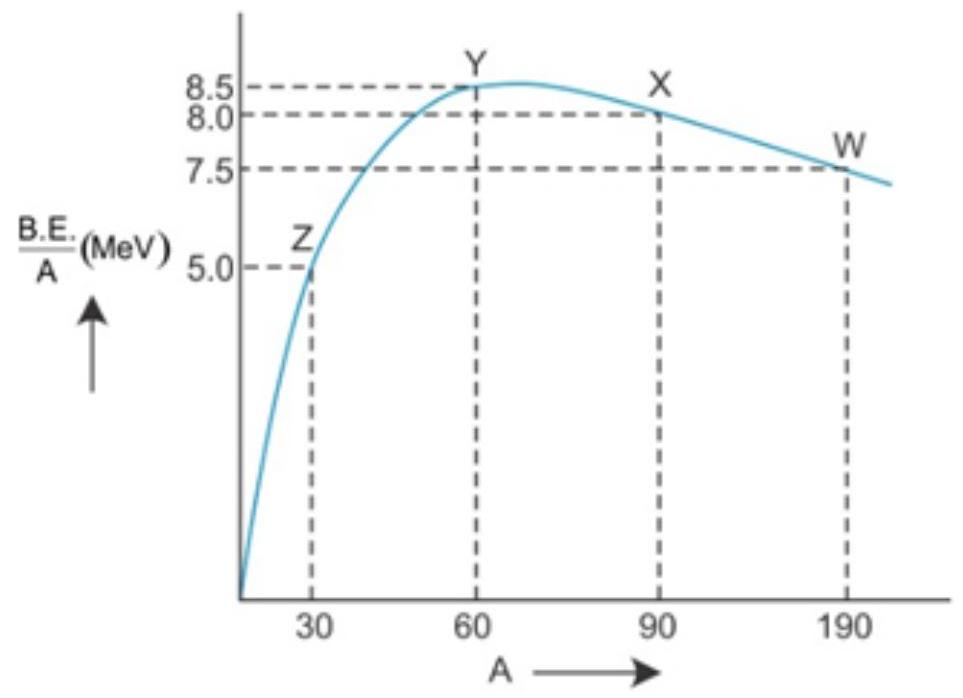
https://asset.sparkl.ac/pb/sparkl-vector-images/img_ncert/mUvmu2d9ndJJeESOG4WRfhelEWflmDggJKihvMFI.png

Question

Using the B.E. per nucleon curve, identify which nucleus suits (i) fission and (ii) fusion. Give a brief reason.

a) Fission-favoured nucleus

b) Fusion-favoured nucleus

Helpful Hints

Hint 1

Heavy nuclei far right, low B.E./A; splitting makes them more stable.

Hint 2

Light nuclei far left gain B.E./A when they merge toward the peak.

Hint 3

Compare how far W and Z lie below the Fe–Ni peak at \(A\approx56\).

Things to Consider

Peak B.E./A at Fe–Ni signifies maximum nuclear stability.
Energy released ∝ Δ(B.E./A)×A; larger gap yields more energy.
Avoid choosing the peak itself for fission or fusion.

Related Concepts

Binding Energy Nuclear Fission Nuclear Fusion

Problem 7 of 10

Analytical Problem Solver

Electromagnetic Waves – Maxwell Correction

Difficulty: Medium Time: 15 min

Problem Statement

A parallel-plate capacitor (area 0.001 m², gap 0.0001 m) is charged so that its voltage rises at \(10^{8}\,\text{V s}^{-1}\). Find the displacement current between the plates.

Given:

Plate area \(A = 0.001\,\text{m}^2\)
Separation \(d = 0.0001\,\text{m}\)
\(\dfrac{dV}{dt}=10^{8}\,\text{V s}^{-1}\), \(\varepsilon_0 = 8.85\times10^{-12}\,\text{F m}^{-1}\)

To Find:

Magnitude of displacement current \(I_d\).

Solution Approaches

Direct Maxwell current

Use \(I_d=\varepsilon_0\frac{A}{d}\dfrac{dV}{dt}\).

Complexity: 1 step

Capacitance first

Find \(C=\varepsilon_0A/d\), then \(I_d=C\dfrac{dV}{dt}\).

Complexity: 2 steps

Electric flux method

Employ \(I_d=\varepsilon_0\dfrac{d\Phi_E}{dt}\) for charging plates.

Complexity: Conceptual

Logical Breakdown

Maxwell correction

Introduces \(I_d\) so Ampere’s law works for charging capacitors.

Capacitance

For parallel plates \(C=\varepsilon_0A/d\).

Voltage change

Charging causes \(\dfrac{dV}{dt}\neq0\) → time-varying electric field.

Numerical substitution

Insert values to obtain \(I_d\) in amperes.

Step-by-Step Solution

Calculate capacitance

\(C=\varepsilon_0\frac{A}{d}=8.85\times10^{-12}\times\frac{0.001}{0.0001}=8.85\times10^{-11}\,\text{F}\).

\(C = 8.85 \times 10^{-11}\,\text{F}\)

Apply charging relation

\(I_d=C\dfrac{dV}{dt}\).

\(I_d = 8.85\times10^{-11}\times10^{8}\)

Compute value

\(I_d = 8.85\times10^{-3}\,\text{A} = 8.85\,\text{mA}\).

Answer: \(8.85\; \text{mA}\)

Key Insights

Displacement current keeps Ampere’s law valid for time-varying fields.
For a capacitor, \(I_d\) matches the conduction current in the connecting wire.
Magnitude depends on area-to-gap ratio and \(\dfrac{dV}{dt}\) during charging.

Analytical Problem Solver

Electrostatic Potential & Capacitance

Difficulty: Medium Time: 15 min

Problem Statement

Two parallel plates are separated by distance \(d\). Insert centrally a slab of
(a) dielectric constant \(k\) and thickness \(t<d\),
(b) metal thickness \(t\). Compare the resulting capacitances with the empty-plate value \(C_0\).

Given:

Plate separation \(d\)
Inserted slab thickness \(t\;(t<d)\)
Dielectric constant \(k\) (case a)

To Find:

Ratios \(C_{\text{dielectric}}/C_0\) and \(C_{\text{metal}}/C_0\).

Solution Approaches

Series model for dielectric

Treat dielectric slab and two air gaps as three capacitors in series.

Key formula: \(\frac{1}{C}=\frac{d- t}{2\varepsilon_0 A}+\frac{t}{k\varepsilon_0 A}\)

Metal reduces gap

Field vanishes inside metal; effective separation becomes \(d-t\).

Capacitance: \(C=\frac{\varepsilon_0 A}{d-t}\)

Check consistency

For \(t\to0\) both results must return to \(C_0\).

Status: Verified

Logical Breakdown

Air gaps

Each gap thickness \((d-t)/2\); permittivity \(\varepsilon_0\).

Dielectric slab

Permittivity \(k\varepsilon_0\); thickness \(t\).

Series combination

Add inverse capacitances to get \(C_{\text{dielectric}}\).

Metal insert

Inside metal \(E=0\) ⇒ only air gap \(d-t\) contributes.

Step-by-Step Solution

Equivalent for dielectric

Use series model: \( \frac{1}{C_d}= \frac{d-t}{2\varepsilon_0 A}+ \frac{t}{k\varepsilon_0 A} \).

\( C_d=\frac{C_0}{\displaystyle 1-\frac{t}{d}+\frac{t}{kd}} \)

Simplify ratio

Divide by \(C_0=\varepsilon_0 A/d\): \( \displaystyle \frac{C_d}{C_0}= \frac{1}{1-\frac{t}{d}+\frac{t}{kd}} \).

Check: \(k\to1\) gives \(C_0\).

Metal case

Effective separation \(d-t\): \(C_m=\frac{\varepsilon_0 A}{d-t}= \frac{C_0}{1-\frac{t}{d}}\).

\( \displaystyle \frac{C_m}{C_0}= \frac{1}{1-\tfrac{t}{d}} \)

Key Insights

Partial dielectric acts like capacitors in series; metal deletes its own thickness.
Capacitance grows with decreasing effective gap: \(C\propto 1/\text{gap}\).
Avoid using \(k\) for metal; its permittivity is effectively infinite.

Analytical Problem Solver

Dual Nature of Radiation & Matter

Difficulty: Medium Time: 15 min

Problem Statement

Three photoelectric I–V curves (A, B, C) for the same metal are given. Identify (i) the two curves with equal light intensity and (ii) the two with equal photon frequency.

Given:

Same metal target and apparatus.
Plateau current = saturation current \(I_{\text{sat}}\).
Voltage where current becomes zero = stopping potential \(V_0\).

To Find:

Pairs with equal intensity and pairs with equal frequency.

Solution Approaches

Compare plateau heights

Equal \(I_{\text{sat}}\) ⇒ equal intensity.

Complexity: O(1)

Compare stopping potentials

Equal \(V_0\) ⇒ equal frequency (\(\nu\)).

Complexity: O(1)

Cross-check results

Use both criteria to avoid misclassification.

Complexity: O(1)

Logical Breakdown

Saturation current

Higher \(I_{\text{sat}}\) → more emitted electrons → greater intensity.

Stopping potential

\(V_0 = \frac{h\nu-\phi}{e}\); depends only on photon frequency.

Intensity inference

Curves with identical plateaus share light intensity.

Frequency inference

Curves with identical \(V_0\) correspond to equal frequency.

Step-by-Step Solution

Measure \(I_{\text{sat}}\)

Read the plateau current for A, B, C and note equal values.

Intensity ∝ \(I_{\text{sat}}\)

Measure \(V_0\)

Locate the voltage where current becomes zero for each curve.

\(eV_0 = h\nu - \phi\)

Draw conclusions

Match curves with equal \(I_{\text{sat}}\) for intensity and equal \(V_0\) for frequency.

State pairs: ( … )

Key Insights

\(I_{\text{sat}}\) signals intensity; it is frequency-independent.
\(V_0\) depends only on photon energy \(h\nu\).
Slopes before saturation carry no information for this analysis.

Analytical Problem Solver

Semiconductor Electronics • Bias Judgement

Difficulty: Medium Time: 15 min

Problem Statement

A cell, ideal diode (anode to +), bulb and switch are in series. Will the bulb glow (a) when the switch is open, (b) when the switch is closed?

Given:

Ideal diode: zero \(R_f\), infinite \(R_r\).
Anode connected to cell’s positive terminal ⇒ forward bias possible.
Bulb glows only when current ≠ 0.

To Find:

Glow status for each switch position.

Solution Approaches

Current-path check

Trace continuity with switch open and closed.

Bias analysis

Determine forward or reverse bias of the ideal diode.

Equivalent circuit view

Replace diode with short (forward) or open (reverse) to predict bulb behaviour.

Logical Breakdown

Switch state

Open ⇒ circuit broken. Closed ⇒ path may exist.

Diode bias

Anode at higher potential gives forward bias; reverse otherwise.

Current flow

Needs closed switch & plus forward-biased diode.

Bulb response

Glows only when \(I \gt 0\).

Step-by-Step Solution

Switch open

Circuit incomplete, current zero, diode bias irrelevant, bulb OFF.

\(I = 0\)

Switch closed

Path complete. Anode is positive, so diode forward biased ⇒ behaves like short.

\(V_D = 0,\; R_D = 0\)

Result

Current flows, bulb glows. If diode were reverse biased, bulb would remain dark.

Bulb ⇒ ON

Key Insights

Ideal diode conducts only under forward bias; blocks completely in reverse bias.
An open switch mimics infinite resistance, stopping current regardless of diode state.
Always judge bulb glow by tracing current path and verifying diode bias together.

Analytical Problem Solver

Current Electricity

Difficulty: Medium Time: 15 min

Problem Statement

A 100 V battery with internal resistance \(r = 1\,\Omega\) sends 10 A through a heater at \(20^{\circ}\text{C}\). When the heater reaches \(320^{\circ}\text{C}\) the current becomes steady. Calculate the power dissipated inside the battery at the higher temperature. Take temperature coefficient of resistance \( \alpha = 4.0 \times 10^{-3}\,^{\circ}\text{C}^{-1} \).

Given:

Battery emf \(E = 100\text{ V}\)
Internal resistance \(r = 1\,\Omega\)
Initial current \(I_0 = 10\text{ A}\) at \(20^{\circ}\text{C}\)
Final temperature \(T = 320^{\circ}\text{C}\)
Temperature coefficient \( \alpha = 4.0 \times 10^{-3}\,^{\circ}\text{C}^{-1}\)

To Find:

Power lost in internal resistance after heating.

Solution Approaches

Direct α-method

Use \(R = R_0[1+\alpha\Delta T]\) to update heater resistance, then compute current and battery loss.

Complexity: Simple math

Graphical I–R analysis

Plot \(I\) vs \(R\) for fixed \(E,r\); read current for new \(R\).

Complexity: Visual

Percent-change shortcut

Estimate current drop using small-change approximation for \(R\) increase.

Complexity: Approximate

Logical Breakdown

Initial heater resistance \(R_0\)

Derived from Ohm’s law using given current and internal resistance.

Temperature rise \(\Delta T\)

\(320^{\circ}\text{C} - 20^{\circ}\text{C} = 300^{\circ}\text{C}\).

New heater resistance \(R\)

Apply \(R = R_0(1+\alpha\Delta T)\) to include temperature coefficient.

Battery loss \(P_r\)

Use \(P_r = I^{2} r\) with updated current to quantify internal resistance power.

Step-by-Step Solution

Compute \(R_0\)

\(R_0 = \frac{E}{I_0} - r = \frac{100}{10} - 1 = 9\,\Omega\).

\(R_0 = 9\,\Omega\)

Update heater resistance

\(R = 9[1 + (4.0\times10^{-3})(300)] = 9 \times 2.2 = 19.8\,\Omega\).

\(R = 19.8\,\Omega\)

Find current & battery loss

\(I = \frac{100}{19.8 + 1} \approx 4.8\,\text{A}\).
\(P_r = I^{2} r \approx (4.8)^{2}(1) \approx 23\,\text{W}\).

\(P_r \approx 23\,\text{W}\)

Key Insights

Resistance rises linearly with temperature for metal heaters: \(R \propto 1+\alpha\Delta T\).
Battery loss depends on internal resistance power \(I^{2}r\); lower current reduces unwanted heating.
Linking temperature coefficient to circuit analysis meets the learning goal: analyse temperature impact on battery efficiency.

Analytical Problem Solver

Electromagnetic Induction – AC Generator Equation

Difficulty: Medium Time: 15 min

Problem Statement

Derive the instantaneous emf \( \varepsilon = N A B \omega \sin \omega t \) for a coil of \(N\) turns and area \(A\) rotating with angular speed \( \omega \) in a uniform magnetic field \(B\).

Given:

Uniform magnetic field \(B\).
Coil with \(N\) turns and area \(A\).
Angular speed \( \omega \); plane makes angle \( \omega t \) with field.

To Find:

Expression for induced emf as a function of time.

Solution Approaches

Faraday derivative

Differentiate \( \Phi = N A B \cos \omega t \) to get emf.

Effort: One derivative

Phasor shift

Emf leads flux by \(90^\circ\); cosine becomes sine.

Effort: Conceptual

Flux-cutting view

Sine arises from component of \(B\) cut per unit time.

Effort: Geometric

Logical Breakdown

Flux expression

\( \Phi(t)= N A B \cos \omega t \).

Differentiate

\( d\Phi/dt = - N A B \omega \sin \omega t \).

Apply Faraday

\( \varepsilon = - d\Phi/dt \).

Result

\( \varepsilon = N A B \omega \sin \omega t \).

Step-by-Step Solution

Write magnetic flux

Flux through coil changes as cosine of angle.

\( \Phi(t)= N A B \cos \omega t \)

Apply Faraday’s law

Induced emf equals negative time rate of flux change.

\( \varepsilon = -\dfrac{d\Phi}{dt} \)

Differentiate & simplify

Derivative converts cosine to sine; negative signs cancel.

\( \varepsilon(t)= N A B \omega \sin \omega t \)

Key Insights

Emf leads magnetic flux by \(90^\circ\); hence sine form.
Sign errors or omitting \(N\) are common pitfalls.
Greater \(N, A, B,\) or \( \omega \) increases generator output.

Analytical Problem Solver

Ray Optics – Right-angled Prism & TIR

Difficulty: Medium Time: 15 min

Problem Statement

A ray just grazes face AC of a right-angled prism. (a) Find the prism’s refractive index. (b) When AC is immersed in a liquid of \(n=\dfrac{2}{\sqrt{3}}\), will the ray undergo total internal reflection or refraction?

Given:

Right-angled prism (\(45^\circ\), \(45^\circ\), \(90^\circ\))
Ray grazes face AC ⇒ angle of refraction \(=90^\circ\)
Initial surrounding: air \((n=1)\); later: liquid \(\displaystyle n=\frac{2}{\sqrt{3}}\)

To Find:

Prism refractive index and the ray’s fate (TIR or refraction) in the liquid.

Solution Approaches

Snell’s law at grazing

Set \(r=90^\circ\) at AC; solve \(n=\sin i/ \sin r\) for the prism.

Complexity: Easy

Critical angle method

Use \(\sin C = \dfrac{n_{\text{out}}}{n_{\text{prism}}}\) with internal angle \(45^\circ\).

Complexity: Easy

Graphical ray tracing

Sketch rays inside the right-angled prism to verify TIR condition.

Complexity: Moderate

Logical Breakdown

Prism geometry

Right-angled prism has \(45^\circ\) faces, so internal incidence on AC is \(45^\circ\).

Snell’s law

At grazing emergence, \(r=90^\circ\) ⇒ \(n_{\text{prism}}=\dfrac{1}{\sin 45^\circ}\).

Critical angle in liquid

With liquid outside, \(\sin C'=\dfrac{n_{\text{liq}}}{n_{\text{prism}}}\).

TIR condition test

If internal angle > critical angle ⇒ TIR; else ray refracts.

Step-by-Step Solution

Find \(n_{\text{prism}}\)

For grazing emergence, internal incidence = \(45^\circ\).

\(n=\dfrac{1}{\sin 45^\circ}= \sqrt{2}\)

Critical angle in liquid

\(\sin C'=\dfrac{n_{\text{liq}}}{n}=\dfrac{\dfrac{2}{\sqrt{3}}}{\sqrt{2}}=\dfrac{2}{\sqrt{6}}\).

\(C' \approx 54^\circ\)

Decide ray’s fate

Internal angle \(45^\circ < C' (54^\circ)\). Condition for TIR unmet.

Ray refracts into liquid; no TIR.

Key Insights

Grazing emergence fixes the internal angle at the critical angle.
Critical angle varies with the surrounding medium: \(\sin C = n_{\text{out}}/n_{\text{in}}\).
Right-angled prisms need \(n \ge \sqrt{2}\) for guaranteed TIR at 45° faces.

Analytical Problem Solver

Atoms – Rutherford Scattering Energy

Difficulty: Medium Time: 15 min

Problem Statement

An \(\alpha\)-particle moves toward a nucleus with speed \(V\) and stops momentarily at closest approach \(d\). What speed is required for a new closest approach of \(d/2\)?

Given:

\(\alpha\)-particle charge \(+2e\), mass \(m\) unchanged
Nuclear charge \(+Ze\)
Initial case: speed \(V\), closest approach \(d\)

To Find:

Required speed \(v\) for closest approach \(d/2\)

Solution Approaches

Energy Conservation

Set initial kinetic energy equal to electrostatic potential energy at minimum distance.

Complexity: Conceptual

Dimensional Reasoning

Recognise \(KE\propto 1/d\) for identical charges; scale speed accordingly.

Complexity: Rapid check

Numerical Substitution

Insert values after deriving the general relation to verify \(v=\sqrt{2}V\).

Complexity: Minimal

Logical Breakdown

Initial Kinetic Energy

\( KE_1=\frac12 mV^2 \)

Electrostatic PE at \(d\)

\( U_1=\frac{1}{4\pi\varepsilon_0}\frac{2Ze^2}{d} \)

Second Scenario PE

\( U_2=\frac{1}{4\pi\varepsilon_0}\frac{2Ze^2}{d/2}=2U_1 \)

Speed Relation

Set \(KE_2=U_2\Rightarrow\frac12 mv^2=2U_1=2KE_1\Rightarrow v=\sqrt{2}V\).

Step-by-Step Solution

Equate Energies (Case 1)

For closest approach \(d\): \( \frac12 mV^2 = \frac{1}{4\pi\varepsilon_0}\frac{2Ze^2}{d} \).

\( KE_1 = U_1 \)

Set Up Case 2

For closest approach \(d/2\): \( \frac12 mv^2 = \frac{1}{4\pi\varepsilon_0}\frac{2Ze^2}{d/2} = 2U_1 \).

\( KE_2 = 2U_1 \)

Take Ratio & Solve

\( \frac{v^2}{V^2} = \frac{KE_2}{KE_1}=2 \Rightarrow v = \sqrt{2}\,V \).

Answer: \( v = \sqrt{2}\,V \)

Key Insights

Closest approach varies inversely with initial kinetic energy in Rutherford scattering.
Halving distance requires doubling the kinetic energy, hence speed increases by \(\sqrt{2}\).
Always compare energies, not forces, to meet the learning outcome.

Key Take-aways

Formula Flash

Prepare a recap sheet. Memorise \(E=\frac{hc}{\lambda}\), \(V=IR\), \(v=u+at\) and similar core relations.

Unit Check

Top thing to remember: always convert to SI; dimensional checks catch errors instantly.

Vector & Sign

Remember directions. Apply right-hand rules and sign conventions to avoid negative surprises.

Diagram & Graph

Neat sketches of circuits, rays or motion graphs communicate logic and save explanation time.

Time Plan

Scan paper quickly, tackle sure shots first, reserve final five minutes for OMR or recheck.

Review & Present

Finish with a clean review—units, significant figures, and margins tidy—so no marks leak.